Part 1: Foundations
Chapter 1: The Signal and the Noise
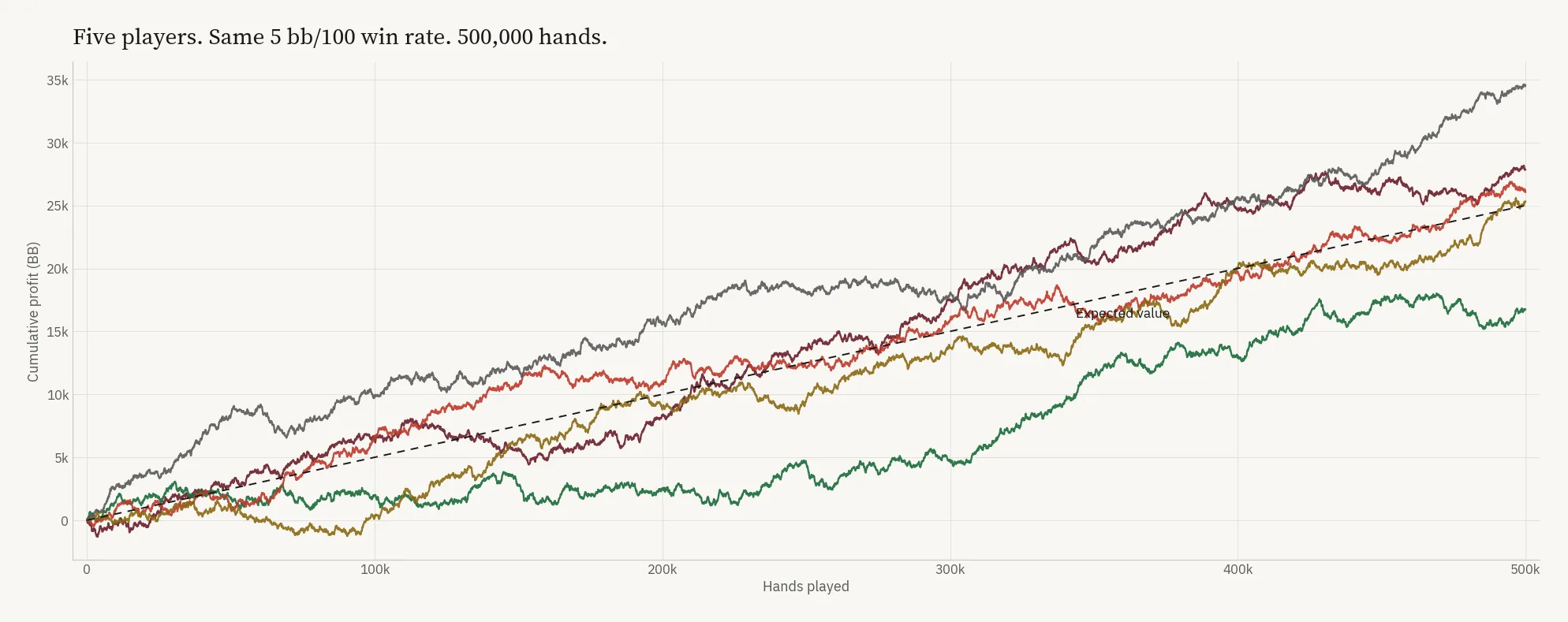
Poker players talk about variance constantly. They say they're "running bad" or "running good," they complain about downswings, they credit heaters. But most players who use the word have an intuitive sense of it rather than a precise one, and that imprecision costs money away from the table: in bankroll decisions, in stake selection, and in the choice to keep playing at all. Making those decisions well requires knowing what variance measures.
A Precise Definition
Variance is a statistical measure of how far individual outcomes spread from the average outcome. In poker, it quantifies how far real outcomes (the cards) stray from expected results (your skill). The related measure, poker standard deviation, is simply the square root of variance and is more intuitive to work with because it's expressed in the same units as your results.
A non-poker example makes this concrete. Imagine two people who commute to work. Person A drives on a highway with no traffic lights. The commute takes 25 to 35 minutes every day, averaging 30 minutes. Person B takes back roads through school zones and construction. The commute takes 15 to 55 minutes, also averaging 30 minutes. Both commuters have the same expected travel time. But Person B has far higher variance. On any given day, Person B's actual experience deviates much further from the average.
The average is the same, but the experience is radically different. Poker results carry the same split between average and experience.
The Two Numbers Behind Every Result
Two numbers govern every poker result: win rate and standard deviation.
Your win rate (measured in big blinds per 100 hands for cash games, or ROI for tournaments) represents your expected earnings per unit of play. It's the signal: the skill edge you bring to the table after all factors including rake.
Your standard deviation (measured in big blinds per 100 hands for cash games) represents the noise: how much your results bounce around that expected value on any given day, week, or month. It captures the combined effect of card distribution, opponent action, pot sizes, and all the other random elements that make poker results unpredictable in the short term.
The defining characteristic of poker is that the noise is enormous relative to the signal. A strong online cash game player might win at 4 bb/100 with a standard deviation of 90 bb/100. The noise is more than 20 times larger than the signal. This ratio is why poker is one of the highest-variance skill games that exist. Chess, go, and most other strategy games don't come close to producing this kind of short-term randomness for a skilled player.
A strong online cash game player might win at 4 bb/100 with a standard deviation of 90 bb/100. The noise is more than 20 times larger than the signal.
This ratio also explains why poker arguments about who is "better" based on results are almost always meaningless. The signal is so faint relative to the noise that it takes an enormous number of hands before skill reliably separates itself from luck.
What Standard Deviation Means in Practice
When a player has a standard deviation of 90 bb/100, it means that over any given 100-hand stretch, the actual result will typically deviate from the expected result by about 90 big blinds. Over 100 hands at NL50 (where a big blind is $0.50), that's $45 of random fluctuation in a session where your expected profit is only $2 (4 bb/100 times $0.50 per bb).
Scale that up. Over 10,000 hands, the standard deviation of your total results is:
SD_total = SD_per_100 * sqrt(number_of_hands / 100)

SD_total = 90 * sqrt(10000 / 100)

SD_total = 90 * 10

SD_total = 900 big blinds
At NL50, 900 big blinds is $450. Your expected profit over 10,000 hands is 400 bb ($200), but the typical deviation from that expectation is $450. You are more likely to end up anywhere in the range from -$250 to +$650 than you are to end up near $200.
That is variance: a measurable, predictable spread of outcomes that dwarfs your edge in the short term.
The Structural Reasons Poker Produces Extreme Variance
Several features of poker combine to produce extreme variance compared to other skill games.
First, individual hand outcomes are largely determined by card distribution and board runout. A player who gets all the money in with 80% equity still loses 20% of the time. Over enough repetitions, those 20% losses cluster into streaks that feel impossible but are statistically inevitable.
Second, pot sizes vary dramatically. A hand where you win 2 big blinds preflop and a hand where you stack someone for 200 big blinds are both "one hand," but their impact on your results differs by a factor of 100. This pot-size variance amplifies the randomness far beyond what you'd see in a game with fixed stakes per decision.
Third, poker is a game of incomplete information. Unlike chess, where the stronger player can often grind out a win through pure technique, poker's hidden information means that even optimal play produces a wide distribution of outcomes on any individual hand.
The result is a game where your skill expresses itself clearly only over very large samples, and "very large" means far more hands or tournaments than most players ever accumulate.
The Normal Distribution and Your Results
Cash game results over large samples approximate a normal distribution, the familiar bell curve. This is a consequence of the central limit theorem: when you add up a large number of independent random outcomes (individual hands), the total converges toward a normal distribution regardless of the shape of the individual hand outcomes.
What this means practically is that the normal distribution's properties can be used to make precise predictions about your results. Given your win rate and standard deviation, you can calculate the probability of finishing a given number of hands with any particular result, positive or negative.
The normal distribution is fully described by two parameters: the mean (your win rate) and the standard deviation. Everything else (the probability of a losing month, the expected length of your worst downswing, the bankroll you need to survive) derives from those two numbers. That's why knowing them, and knowing them accurately, matters so much.
A Worked Example
Consider a solid online NLHE 6-max player at NL50 ($0.25/$0.50 blinds, $50 max buy-in):
Win rate: 5 bb/100
Standard deviation: 80 bb/100
Sample: 100,000 hands (about four months of part-time play)
Expected profit over 100,000 hands:
EV = (WR / 100) * number_of_hands * bb_value

EV = (5 / 100) * 100,000 * $0.50

EV = $2,500
Standard deviation of total results over 100,000 hands:
SD_total = SD_per_100 * sqrt(hands / 100) * bb_value

SD_total = 80 * sqrt(100,000 / 100) * $0.50

SD_total = 80 * 31.62 * $0.50

SD_total = $1,265
The 95% confidence interval for total results:
Lower bound = $2,500 - (1.96 * $1,265) = $2,500 - $2,479 = $21

Upper bound = $2,500 + (1.96 * $1,265) = $2,500 + $2,479 = $4,979
This player expects to win $2,500 over 100,000 hands. But 95% of the time, the actual result will fall somewhere between roughly breaking even and winning nearly $5,000. And 5% of the time, the result will fall outside even that wide range.
A player who runs this through the Primedope poker variance calculator (https://www.primedope.com/poker-variance-calculator/), a poker variance simulator that generates 20 independent outcome paths from your parameters, will see that most paths look nothing like the smooth expected value line. Some climb steadily, some plunge into long downswings before recovering, and a few end up in negative territory despite 100,000 hands of play by a winning player.
Chapter 2: The Core Formulas
The formulas you need are here: expected value, standard deviation, confidence intervals, risk of ruin, minimum bankroll, and sample size. Each one comes with a worked dollar example. Use this chapter as a reference.
Expected Value in Dollars
Your win rate tells you how much you expect to earn per hand on average. Converting it to dollars is simple:
Hourly EV = (WR / 100) * hands_per_hour * bb_value
Example: 4 bb/100 at NL100 ($0.50/$1.00), playing 500 hands per hour (multi-tabling)
Hourly EV = (4 / 100) * 500 * $1.00 = $20/hour
Monthly EV (100 hours) = $2,000

Annual EV (1,200 hours) = $24,000
These numbers represent what happens on average over the long run. They are not predictions for any individual month. The difference between what you expect and what you experience in any given period is the entire subject of this guide.
Standard Deviation: What It Is and Where to Find Yours
Your tracking software reports this number. In PokerTracker 4, it's under your cash game stats in the More Detail tab, labeled "Std Dev" in bb/100. Hand2Note shows it in the player summary panel. If you play on a site that provides hand histories, you can import them into either tool and the software calculates it automatically.
Typical standard deviations by format:
| Game Type | Typical SD Range (bb/100) |
|---|---|
| NLHE 6-max | 75-120 |
| NLHE Full Ring | 60-80 |
| NLHE Heads-Up | 100-140 |
| PLO 6-max | 120-160 |
| PLO Full Ring | 100-140 |
| Live NLHE (1/2 to 5/10) | 120-160 |
If your standard deviation falls significantly outside these ranges, it may indicate an unusual playing style. Very loose-aggressive players tend toward higher SDs, while tight-passive players tend lower. Neither is inherently better, but the number directly affects your bankroll requirements and the severity of your downswings.
Confidence Intervals: The 68/95/99.7 Rule
For a normally distributed result (which cash game results approximate over large samples), the following rules apply:
Your actual result falls within one standard deviation of the expected value with 68% probability, within 1.96 standard deviations with 95% probability, and within three standard deviations with 99.7% probability.
Applied to poker:
Player: 3 bb/100 win rate, 90 bb/100 SD, 200,000 hands at NL50 ($0.50 bb)
Expected profit = (3/100) * 200,000 * $0.50 = $3,000

SD of total results = 90 * sqrt(200,000/100) * $0.50 = 90 * 44.72 * $0.50 = $2,012
68% confidence interval: $3,000 +/- $2,012 = [$988 to $5,012]

95% confidence interval: $3,000 +/- $3,944 = [-$944 to $6,944]

99.7% confidence interval: $3,000 +/- $6,037 = [-$3,037 to $9,037]
A 3 bb/100 winner at NL50 who plays 200,000 hands has a roughly 7% chance of finishing with a loss, and that's over a sample that might represent an entire year of part-time play. You can model your own parameters using the Primedope poker variance calculator (https://www.primedope.com/poker-variance-calculator/), which displays these intervals graphically. One note on methodology: this guide uses the precise statistical multipliers (1.96 for 95%, 1.00 for 68%) while the calculator uses the common rounded approximations (2.0 for 95%, 1.0 for 70%). The practical difference is negligible, but if you compare the calculator's output to the worked examples here, this explains any small discrepancies.
Risk of Ruin
Risk of ruin (RoR) is the probability that you will lose your entire bankroll before it grows indefinitely, assuming you play at the same stakes with the same win rate forever. The formula for a cash game player is:
Risk of Ruin = e^(-2 * WR * BR / SD^2)
Where:

  WR = win rate in bb/100

  BR = bankroll in big blinds

  SD = standard deviation in bb/100

  e  = Euler's number (approximately 2.718)
Worked example:
WR = 3 bb/100

BR = 5,000 bb (50 buy-ins at NL100)

SD = 85 bb/100
RoR = e^(-2 * 3 * 5000 / 85^2)

RoR = e^(-30,000 / 7,225)

RoR = e^(-4.15)

RoR = 1.6%
A 50-buy-in bankroll gives this player a 1.6% chance of going broke, assuming the win rate and standard deviation remain stable and the player stays at the same stakes indefinitely. In practice, most players move down when their bankroll shrinks, which reduces the actual risk of ruin below what the formula predicts. The formula gives you the worst-case baseline. Change the bankroll to 30 buy-ins (3,000 bb) and the risk of ruin jumps to 8.3%, a very different proposition. The Primedope poker variance calculator (https://www.primedope.com/poker-variance-calculator/) computes risk of ruin automatically for any win rate, standard deviation, and bankroll size you enter.
Minimum Bankroll Calculation
The inverse question: how large a bankroll do you need for a given risk tolerance? Solving the risk of ruin formula for bankroll:
BR = -SD^2 * ln(RoR_target) / (2 * WR)
Where:

  ln = natural logarithm

  RoR_target = acceptable risk of ruin (e.g., 0.05 for 5%)
Example: A player with 3 bb/100 win rate and 85 bb/100 SD who wants less than 5% risk of ruin:
BR = -(85^2) * ln(0.05) / (2 * 3)

BR = -7,225 * (-2.996) / 6

BR = 21,644 / 6

BR = 3,607 big blinds
That's approximately 36 buy-ins. For a 1% risk of ruin, the same calculation yields about 55 buy-ins. The numbers grow quickly as your win rate shrinks or your standard deviation increases, which is why PLO players and players at tough, high-stakes games need substantially deeper bankrolls than the standard "30 buy-ins" rule suggests. Use the Primedope poker variance calculator as a poker bankroll calculator by plugging your parameters into the risk of ruin formula above.
The Sample Size Problem
The most common question in poker bankroll planning, and the one players get most consistently wrong: how many poker hands does it take to determine your win rate? For most players, the answer is more hands than they will ever play.
The standard error of your observed win rate is:
SE = SD / sqrt(number_of_hands / 100)
Where:

  SE = standard error in bb/100

  SD = standard deviation in bb/100
This tells you the margin of error on your win rate estimate. The 95% confidence interval for your true win rate is approximately your observed win rate plus or minus 1.96 standard errors.
Example: SD = 90 bb/100
At 25,000 hands:  SE = 90 / sqrt(250) = 5.69 bb/100

At 50,000 hands:  SE = 90 / sqrt(500) = 4.02 bb/100

At 100,000 hands: SE = 90 / sqrt(1000) = 2.85 bb/100

At 250,000 hands: SE = 90 / sqrt(2500) = 1.80 bb/100

At 500,000 hands: SE = 90 / sqrt(5000) = 1.27 bb/100
At 100,000 hands, if your observed win rate is 4 bb/100, your true win rate is somewhere between -1.6 and 9.6 bb/100 (95% confidence). That range covers both an excellent player and a losing one, and the sample cannot tell you which you are.
The following table shows the 95% confidence margin at various sample sizes for a player with 90 bb/100 standard deviation:
| Hands Played | 95% Margin (+/-) | What It Means |
|---|---|---|
| 25,000 | 11.2 bb/100 | Essentially meaningless |
| 50,000 | 7.9 bb/100 | Can distinguish big winner from big loser |
| 100,000 | 5.6 bb/100 | Can distinguish winner from loser, roughly |
| 250,000 | 3.5 bb/100 | Reasonable estimate emerging |
| 500,000 | 2.5 bb/100 | Solid estimate for most purposes |
| 1,000,000 | 1.8 bb/100 | High confidence |
Most recreational and semi-professional players will never have a large enough poker sample size to know their true win rate with precision. A player who puts in 50,000 hands per year would need five years to reach 250,000 hands, and by then their game, the player pool, and the stakes have all likely changed. Knowing whether you are a winning poker player, with genuine confidence, requires more data than most players ever accumulate. The sample requirement is a structural feature of the game; no amount of determination changes it.
Chapter 3: Short-Term Results Tell You Almost Nothing
The oldest argument in poker is whether poker is luck or skill. The answer is both, in specific proportions that change depending on the time frame. Over a single session, luck decides nearly everything. Over 100,000 hands, skill is the primary driver. The math in Chapter 2 tells you exactly where you are on that spectrum at any sample size. Most players are operating in a zone where luck still carries far more weight than they believe.
The Core Problem
At 50,000 hands, which represents roughly 100 hours of 8-tabling online, the 95% confidence interval on your win rate spans approximately 16 bb/100. A player showing a 5 bb/100 profit rate over that sample could just as easily be a breakeven player who ran well, or a 10 bb/100 crusher who ran normally. The observed number is compatible with such a wide range of true abilities that it cannot reliably distinguish between them.
Most players understand this intellectually and reject it emotionally. When you're in the middle of a 30,000-hand downswing, the abstract knowledge that "this is within normal variance" provides cold comfort. And when you're on a 30,000-hand heater, you're unlikely to question whether your recent success might be mostly luck. The asymmetry is revealing: players attribute bad runs to variance and good runs to skill. The math says neither attribution is justified at these sample sizes.
A 50,000-Hand Downswing Is Routine for a Winning Player
Take a player with a true win rate of 4 bb/100 and a standard deviation of 90 bb/100. Over 50,000 hands, their expected profit is 2,000 big blinds. But the standard deviation of their total result over that stretch is approximately 2,012 big blinds.
EV = (4 / 100) * 50,000 = 2,000 bb

SD_total = 90 * sqrt(50,000 / 100) = 90 * 22.36 = 2,012 bb

95% range of outcomes: 2,000 +/- 3,944 bb = [-1,944 bb to +5,944 bb]
This means a 4 bb/100 winner has roughly a 16% chance of being in the red after 50,000 hands. Nearly one in six 50,000-hand stretches will show a loss even though the player is winning at a healthy rate.
A 4 bb/100 winner has roughly a 16% chance of being in the red after 50,000 hands. Nearly one in six stretches of that length will show a loss.
A 50,000-hand poker downswing is a routine event for a winning player with normal variance.
A 50,000-Hand Heater Is Not Evidence Either
The same math works in reverse. A breakeven player (0 bb/100 true win rate) with 90 bb/100 standard deviation will show a positive result over 50,000 hands approximately 50% of the time, by definition, since the expected result is zero and outcomes are roughly symmetric.
A player with a true win rate of -2 bb/100, an actual losing player, has approximately a 31% chance of showing a profit over 50,000 hands at 90 bb/100 standard deviation. Nearly one-third of the time, a losing player will look like a winner over a sample that represents months of play.
This is why the poker world is full of players who "used to be winning players" before things "changed." Some of them did experience a genuine decline in edge. But some of them were never winning players to begin with. They just ran well for long enough to believe they were.
The Danger of Results-Based Thinking
The practical consequence of insufficient sample sizes is that players constantly make decisions based on data that doesn't support those decisions.
A player runs at 8 bb/100 over 30,000 hands and decides they're ready to move up in stakes. The move-up is based on a win rate estimate that carries a margin of error of plus or minus 10 bb/100. They might be a 0 bb/100 player at their current level, and now they're playing higher stakes where the games are tougher and their (possibly non-existent) edge shrinks further.
A player goes through a 40,000-hand breakeven stretch and concludes their strategy isn't working. They make wholesale changes to their game, tightening up, changing bet sizes, abandoning profitable lines, all based on a sample that tells them almost nothing. The changes might fix actual leaks, or they might destroy real edges. At 40,000 hands, you can't tell which.
A player runs at 2 bb/100 over 100,000 hands and concludes they can't beat the stakes. They either drop down or quit. But 2 bb/100 over 100,000 hands is consistent with a true win rate of 5 bb/100 or higher. They might be giving up on a profitable situation because of a sample that simply hasn't converged yet.
The correct approach is to separate results from analysis. Use your database to study specific decisions: are your 3-bet ranges correct? Are you value-betting thin enough on rivers? Are you folding too much to aggression? These hand-by-hand analyses are valid at any sample size because they evaluate the decision rather than the outcome. Base strategic changes on your play in specific, reviewable spots, never on your overall win rate over 50,000 hands.
What You Can Trust at Various Sample Sizes
Rather than trusting your bottom-line results, here is what different sample sizes can tell you:
At 10,000 hands, you can identify gross leaks (open-limping every hand, never 3-betting, calling every river bet) from your stat profiles. You cannot draw any meaningful conclusion about your win rate.
At 50,000 hands, you can start to trust broad statistical tendencies. If your VPIP is 35 in a 6-max game, that's a reliable indicator of a too-loose preflop strategy regardless of your results. You still cannot trust your win rate to distinguish between winning and losing.
At 100,000 hands, your win rate estimate has a margin of error of roughly 5.6 bb/100 (at 90 bb/100 SD). You can begin to distinguish between clear winners and clear losers, but the grey zone is wide. A player showing 3 bb/100 could easily be anywhere from breakeven to very strong.
At 500,000 hands, your win rate margin narrows to about 2.5 bb/100. This is where you can start making real conclusions. If you're showing 4 bb/100 over half a million hands, you're almost certainly a winning player, though your exact win rate still has meaningful uncertainty.
Results do matter, over the very long run. But "the long run" is much longer than almost anyone intuitively believes, and making decisions as if you've reached it when you haven't is one of the most expensive mistakes in poker, paid in the bankroll and stakes decisions made away from the table.
If you are running bad at poker and trying to determine whether variance or your actual play is responsible, the calculator is the right starting point. Enter your observed win rate, your standard deviation, and the number of hands you've played into the Primedope poker variance calculator (https://www.primedope.com/poker-variance-calculator/). The output tells you the full range of outcomes consistent with your data, and how often a player with your stated win rate would produce a result as bad as yours. If your result falls comfortably within the expected range, you are running bad. If it sits outside the range, something else has changed.
Part 2: Cash Game Variance
Chapter 4: Cash Game Variance by the Numbers
The foundations from Part 1 apply to all poker formats, but the specifics differ dramatically between cash games and tournaments. This chapter translates the general framework into concrete numbers for cash game players across formats, stakes, and settings.
Standard Deviations by Format
Not all cash games produce the same variance. The format you play determines your standard deviation more than almost any other factor, and the differences are large enough to require fundamentally different bankroll strategies.
| Game Type | Typical SD Range (bb/100) | Primary Drivers |
|---|---|---|
| NLHE Full Ring (9-max) | 60-80 | Fewer hands played, tighter ranges, smaller average pots |
| NLHE 6-max | 75-120 | More hands played per orbit, wider ranges, more postflop aggression |
| NLHE Heads-Up | 100-140 | Every hand contested, large pots relative to stack depth |
| PLO 6-max | 120-160 | Closer equities, more multiway action, larger average pots |
| PLO Full Ring | 100-140 | Same equity dynamics as PLO 6-max, somewhat fewer contested pots |
| Live NLHE (1/2 to 5/10) | 120-160 | Deeper effective stacks, more multiway pots, more limping and calling |
Compare NLHE full ring at 70 bb/100 with PLO 6-max at 140 bb/100. Doubling the standard deviation roughly quadruples the variance (since variance is the square of standard deviation), which means the PLO player needs approximately four times the bankroll to achieve the same risk of ruin, all else being equal.
How Stake Level Affects Variance
A common misconception is that higher stakes mean higher variance. In absolute dollar terms, this is obviously true. But in terms of standard deviation measured in big blinds per 100 hands, the relationship is more complicated.
At micro stakes (NL2 through NL25), player pools tend to be looser and more passive. This creates larger average pots through more calling and less folding, which pushes standard deviations toward the higher end of the range. However, win rates at micro stakes also tend to be higher for competent players, because the opposition is weaker. The higher win rate partially compensates for the higher variance.
At mid stakes (NL50 through NL200), the games tighten up. Players are more aggressive but also more selective, which can moderate pot sizes in some configurations. Standard deviations in this range tend to cluster in the middle of the typical range for each format.
At high stakes (NL500 and above), the games become more adversarial. Aggressive 3-betting and 4-betting sequences create large preflop pots, and postflop play involves more check-raises and overbets. Standard deviations can be high, but the more important factor is that win rates compress. A 2 bb/100 edge at NL1000 produces far more precarious variance dynamics than a 5 bb/100 edge at NL50, even if the standard deviations are similar.
Live vs. Online: A Different Variance Experience
Live and online poker variance differ in structure, and the difference feeds directly into live poker bankroll requirements.
Live games typically produce higher standard deviations per 100 hands. The primary drivers are deeper effective stacks (many live games play 200bb+ deep as a matter of course), more multiway pots (live players call more and fold less preflop), and more irregular bet sizing that creates larger pots. A live 1/2 or 2/5 NLHE game commonly produces standard deviations of 120 to 160 bb/100.
However, live players see far fewer hands per hour. A typical live game deals 25 to 35 hands per hour, compared to 60 to 80 hands per hour per table online (and most online players multi-table). The result is that a live player's monthly results, measured in total big blinds won or lost, have a lower total standard deviation than an online player's monthly results despite the higher per-hand variance. The live player simply hasn't accumulated enough hands for the variance to compound.
The practical implication: live players experience wilder individual sessions (because each session is a small sample at high SD) but smoother monthly and yearly results (because the total hand count stays low). Online players experience the opposite. Individual sessions feel more predictable, but over 50,000 or 100,000 hands per month, the cumulative variance can produce extended downswings that a live player would rarely encounter in terms of total hands.
Both settings demand adequate bankrolls, but the texture of the variance feels different. Live players need to be psychologically prepared for individual sessions where they lose five or more buy-ins through no fault of their own. Online players need to be prepared for multi-week or multi-month stretches where the graph trends relentlessly downward.
Multi-Tabling: Volume vs. Quality
Online cash game players face a trade-off that doesn't exist in live poker: how many tables to play simultaneously. Multi-tabling increases hands per hour, which speeds convergence toward your true win rate and increases total expected earnings per session. But it typically reduces win rate per table because attention is split across more simultaneous decisions.
The variance math cuts in multiple directions here. Playing 8 tables at 3 bb/100 produces a lower standard deviation of total hourly results than playing 2 tables at 5 bb/100, because the larger hand count smooths things out. But the per-hand win rate is lower, which means the bankroll needs to be larger relative to the expected earnings, and the risk of ruin is higher per hand played.
The practical framework: add tables until you notice your win rate per table declining in your database over a meaningful sample (at least 30,000 hands at the new table count). The right table count is the one where your total hourly EV peaks, rather than the one where your per-table win rate peaks. But if you're in a downswing, reducing tables to protect per-table win rate is often the higher-EV play, as discussed in Chapter 11.
Four Player Profiles
The following profiles represent realistic scenarios across different stakes and commitment levels. For each, the math shows the expected results, the realistic range of outcomes, and the bankroll required. All figures assume play over one year.
Profile 1: The NL10 Grinder
Win rate: 3 bb/100
Standard deviation: 85 bb/100
Hands per year: 200,000
Big blind value: $0.10
Expected annual profit: (3/100) * 200,000 * $0.10 = $600
SD of annual results: 85 * sqrt(200,000/100) * $0.10 = 85 * 44.72 * $0.10 = $380
95% confidence interval: $600 +/- $745 = [-$145 to $1,345]
Probability of a losing year: approximately 6%
Minimum bankroll at 5% RoR: BR = -(85^2) * ln(0.05) / (2 * 3) = 3,607 bb = $361 (approximately 36 buy-ins)
Expected worst downswing over 200,000 hands: approximately 2,500 to 3,500 bb ($250 to $350)
This player is grinding for learning and incremental profit. The dollar amounts are small, but the variance dynamics are real. A $350 downswing at NL10 is psychologically significant for a player whose entire bankroll might be $400 to $500.
Profile 2: The NL50 Semi-Pro
Win rate: 4 bb/100
Standard deviation: 90 bb/100
Hands per year: 400,000
Big blind value: $0.50
Expected annual profit: (4/100) * 400,000 * $0.50 = $8,000
SD of annual results: 90 * sqrt(400,000/100) * $0.50 = 90 * 63.25 * $0.50 = $2,846
95% confidence interval: $8,000 +/- $5,578 = [$2,422 to $13,578]
Probability of a losing year: less than 1%
Minimum bankroll at 5% RoR: BR = -(90^2) * ln(0.05) / (2 * 4) = 3,033 bb = $1,517 (approximately 30 buy-ins)
Expected worst downswing over 400,000 hands: approximately 4,000 to 6,000 bb ($2,000 to $3,000)
This player expects to make $8,000 over the year, but a $3,000 downswing is well within normal range. If the player's bankroll is $2,000 and they experience even a moderate downswing early, the math puts them in a difficult position before the long-term edge has time to express itself.
Profile 3: The NL200 Pro
Win rate: 2.5 bb/100
Standard deviation: 95 bb/100
Hands per year: 600,000
Big blind value: $2.00
Expected annual profit: (2.5/100) * 600,000 * $2.00 = $30,000
SD of annual results: 95 * sqrt(600,000/100) * $2.00 = 95 * 77.46 * $2.00 = $14,717
95% confidence interval: $30,000 +/- $28,845 = [$1,155 to $58,845]
Probability of a losing year: approximately 2%
Minimum bankroll at 5% RoR: BR = -(95^2) * ln(0.05) / (2 * 2.5) = 5,407 bb = $10,815 (approximately 54 buy-ins)
Expected worst downswing over 600,000 hands: approximately 8,000 to 12,000 bb ($16,000 to $24,000)
The expected profit is $30,000, but the 95% confidence interval nearly touches zero on the low end. A professional player relying on this income could have a year where they barely break even despite playing well for 600,000 hands. The expected worst downswing of $16,000 to $24,000 represents a period where the player's bankroll is being drained while their income has stalled or gone negative. At this level, the bankroll needs to absorb the variance and the player's living expenses simultaneously.
Profile 4: The PLO200 Player
Win rate: 5 bb/100
Standard deviation: 140 bb/100
Hands per year: 300,000
Big blind value: $2.00
Expected annual profit: (5/100) * 300,000 * $2.00 = $30,000
SD of annual results: 140 * sqrt(300,000/100) * $2.00 = 140 * 54.77 * $2.00 = $15,336
95% confidence interval: $30,000 +/- $30,059 = [-$59 to $60,059]
Probability of a losing year: approximately 2.5%
Minimum bankroll at 5% RoR: BR = -(140^2) * ln(0.05) / (2 * 5) = 5,872 bb = $11,743 (approximately 59 buy-ins)
Expected worst downswing over 300,000 hands: approximately 10,000 to 15,000 bb ($20,000 to $30,000)
The PLO player has a higher win rate than the NL200 pro (5 bb/100 vs. 2.5 bb/100) and the same expected annual profit. But the 140 bb/100 standard deviation changes the character of the experience entirely. The 95% confidence interval spans over $60,000 from worst to best case. The required bankroll is 59 buy-ins, nearly double what a comparable NLHE player needs. And the expected worst downswing of $20,000 to $30,000 means this player should be prepared to weather a period where their bankroll drops by an amount equal to their entire annual expected earnings.
Downswing depth estimates throughout this guide are derived from Monte Carlo simulation rather than the closed-form formulas presented in Part 1. You can simulate your own parameters, including PLO variance scenarios, using the Primedope poker variance calculator (https://www.primedope.com/poker-variance-calculator/) to see the full distribution of drawdown depths for your specific situation.
Chapter 5: Rake, the Hidden Variance Amplifier
Every worked example in this guide uses win rates measured after rake. Rake reduces your profits and degrades your variance profile, and the two effects compound over time.
Your True Win Rate Is Your Win Rate After Rake
A player who wins 5 bb/100 before rake at a site that charges 8 bb/100 in effective rake (including the portion of pots taken as rake, adjusted for any rakeback or rewards) is a -3 bb/100 loser. Every calculation in this guide, every bankroll requirement, every risk of ruin estimate, must be performed using the win rate after all rake costs are subtracted.
This seems obvious when stated directly, but many players track their "win rate" as the number reported by their tracking software without thinking carefully about whether that number already includes rake. In most tracking software, the win rate displayed does include rake paid. But it does not include rakeback received, bonus money earned, or loyalty rewards credited outside the hand history. The true after-rake win rate requires manual adjustment. If your site offers rakeback or a rewards program, add the effective value in bb/100 to your tracked win rate before running any variance calculations. For example, if your tracking software shows 3 bb/100 and your rakeback is worth approximately 1 bb/100, your true after-rake win rate for variance modeling purposes is 4 bb/100. This is the number you enter into the Primedope poker variance calculator (https://www.primedope.com/poker-variance-calculator/).
How Rake Varies Across Sites
Choosing among poker sites is a rake decision as much as a game selection decision. The lowest-rake poker sites charge 2 to 3 bb/100 less than the highest-rake alternatives at the same stakes, and that gap changes your entire variance profile. The effective rake you pay depends on the site, the stakes, the pot sizes, and the reward structures.
At the low-to-mid stakes, sites like CoinPoker charge competitive base rake at stakes where the cap rarely binds. Its flat 15% daily rakeback ended in July 2026, so effective rake now depends on variable CoinRewards leaderboard finishes rather than on a published rate.
At higher stakes, the picture shifts. Sites like ACR Poker become more competitive on rake at NL500 and above, where their rake caps and reward structure can produce lower effective costs than sites that are cheaper at lower levels.
GGPoker uses a "net rake" system where only net pot contributions count toward the rake calculation, which benefits some player types and disadvantages others. PokerStars offers modest rewards (roughly 5% equivalent for most players). Ozoon (formerly Bovada) and Ignition charge moderate rake but offer anonymous tables, which creates softer table dynamics that may compensate through a higher pre-rake win rate.
The specifics change over time as sites adjust their structures, which is why running your own comparison using the Primedope Rake Calculator (https://www.primedope.com/online-poker-rake-comparison-rake-calculator/) is worth doing periodically. The calculator draws from a database of 645 data points across 18 networks and is the most complete public rake comparison available.
The Compounding Effect of Rake on Variance
Rake belongs in a variance guide because reducing your effective win rate by even 1 bb/100 has cascading effects on your entire variance profile.
Consider two identical players: same skill level, same standard deviation of 90 bb/100, same volume of 400,000 hands per year at NL100 ($1.00 big blind). The only difference is the rake environment.
Player A: Effective win rate 4 bb/100 (lower-rake site)
Expected annual profit: $16,000
Minimum bankroll at 5% RoR: 3,033 bb ($3,033)
Risk of ruin at 40 buy-ins (4,000 bb): 1.9%
Player B: Effective win rate 2 bb/100 (higher-rake site)
Expected annual profit: $8,000
Minimum bankroll at 5% RoR: 6,066 bb ($6,066)
Risk of ruin at 40 buy-ins (4,000 bb): 13.9%
The 2 bb/100 difference in effective rake cuts Player B's expected income in half. But the damage to the variance profile is even worse. Player B needs double the bankroll to achieve the same risk of ruin. At the same 40 buy-in bankroll, Player B's risk of ruin is more than seven times higher.
The downstream effects compound further. Player B's expected worst downswing is longer and deeper, which means more time playing at reduced confidence, more temptation to move down in stakes (forfeiting expected income), and more psychological pressure from watching the bankroll erode. Beyond the extra income, the 2 bb/100 in rake savings shortens Player A's downswings, reduces the required bankroll, lowers the risk of ruin, and makes the career more sustainable.
This is why game selection and site selection are core bankroll management decisions. A player who spends hours studying solver outputs to eke out an extra 0.5 bb/100 in win rate but never compares the rake structure of their site to alternatives is optimizing the wrong variable.
Chapter 6: Bankroll Management for Cash Games
Poker bankroll management is where the theory from the previous chapters meets the decisions you make with your money. Most players follow rules of thumb (30 buy-ins for NLHE, 50 for PLO) without knowing what those rules assume or where they fail. The numbers below are derived from the actual formula, so you can see exactly what risk you are accepting at any bankroll size.
What the Common Rules of Thumb Assume
The "20 buy-in" rule assumes a relatively high win rate (5+ bb/100), moderate standard deviation, and a willingness to accept meaningful risk of ruin (roughly 10% or higher). It's a reasonable starting point for a strong player at micro stakes who can reload if things go wrong.
The "30 buy-in" rule corresponds to roughly 3 to 5% risk of ruin for a solid winner (3 to 4 bb/100) at standard NLHE 6-max variance. This is the most commonly cited number and works well for a range of realistic scenarios.
The "50 buy-in" rule is appropriate for players with thinner edges (1 to 2 bb/100), higher standard deviations (PLO, heads-up), or a very low risk tolerance. It also makes sense for professional players who cannot easily reload, since going broke has career consequences beyond the dollar amount.
None of these rules are "right" or "wrong" in isolation. Any bankroll management poker strategy built on a rule of thumb without knowing the underlying assumptions is guesswork. The following table replaces the guesswork with the actual risk of ruin for various bankroll sizes, assuming a standard deviation of 90 bb/100:
| Bankroll (buy-ins) | Win Rate 2 bb/100 | Win Rate 3 bb/100 | Win Rate 4 bb/100 | Win Rate 6 bb/100 |
|---|---|---|---|---|
| 20 | 37.3% | 22.7% | 13.9% | 5.2% |
| 30 | 22.7% | 10.8% | 5.2% | 1.2% |
| 40 | 13.9% | 5.2% | 1.9% | 0.27% |
| 50 | 8.5% | 2.5% | 0.72% | 0.06% |
| 75 | 2.5% | 0.39% | 0.06% | < 0.01% |
A player with a 2 bb/100 win rate and 20 buy-ins has a 37% chance of going broke. A bankroll that size is closer to a coin flip than a career plan. The same player with 50 buy-ins drops to 8.5% risk, which means roughly one in twelve players in this situation will go broke despite having a real edge.
The Kelly Criterion, Simplified
The Kelly Criterion is a formula from information theory that tells you the optimal bet size to maximize long-term growth rate. Applied to poker, it suggests the stakes at which your bankroll grows fastest relative to the risk taken.
The simplified Kelly fraction for poker is:
Optimal stakes = (WR * BR) / SD^2
Where:

  WR = win rate in bb/100

  BR = current bankroll in big blinds

  SD = standard deviation in bb/100
In practice, this formula suggests that your current bankroll divided by the Kelly number gives you the maximum stakes you should play. Most professional players use half-Kelly or less, meaning they play at stakes roughly half (or lower) of what the Kelly formula suggests. The reason is that full Kelly is extremely aggressive and produces wild bankroll swings. Half-Kelly sacrifices some growth rate for substantially smoother results.
The practical version: if the Kelly formula says you're rolled for NL200, consider playing NL100 or NL50 to prioritize bankroll stability over maximum growth. The compounding benefits of never going broke and never having to move down outweigh the slightly faster growth rate at higher stakes.
Moving Up and Moving Down
When to move up in poker stakes is one of the most emotion-corrupted decisions in the game. Players move up after heaters, when the bankroll has grown but the underlying win rate hasn't been proven at the higher level. They refuse to move down during downswings, when the bankroll no longer supports the current stakes. Both mistakes have the same root cause: using recent results instead of the math.
A reasonable framework for moving up: you should have the minimum bankroll for the next level (at your target risk of ruin) AND a demonstrated win rate at your current level over a meaningful sample (at least 100,000 hands). Moving up without both conditions met is a shot-take, and it belongs under the shot-taking rules later in this chapter.
For moving down: if your bankroll drops below the minimum for your current stakes at your target risk of ruin, move down immediately, without negotiating with yourself or promising to "win it back." The math is unambiguous. Playing at stakes your bankroll cannot support increases your risk of ruin, and ruin is the one outcome bankroll management exists to prevent.
The Cost of Being Underrolled
Beyond the risk of going broke, playing underrolled costs expected lifetime earnings in a subtler way.
Consider two paths for the same player (4 bb/100 winner, 90 bb/100 SD at NL100):
Path A: starts with 40 buy-ins ($4,000), plays NL100 continuously.
Path B: starts with 15 buy-ins ($1,500), plays NL100, goes broke after a moderate downswing, reloads for $1,500, goes broke again, eventually rebuilds with a third reload.
Player B's expected total cost of going broke twice (including the time spent rebuilding from zero and the sessions played at reduced confidence while short-stacked) runs to thousands of dollars in foregone earnings over a year. The $2,500 "saved" by starting with the smaller bankroll is wiped out several times over by the cost of the ruin events.
The mathematically optimal approach is to start at the highest stakes your bankroll supports at an acceptable risk of ruin, and move up only when the bankroll grows to support the next level. Patience in bankroll building is the highest-EV strategy over a career.
Shot-Taking: A Disciplined Framework
Shot-taking, playing occasionally at stakes above your current bankroll level, can be rational when structured properly.
The framework: set aside a "shot" allocation of 5 buy-ins at the next level from your current bankroll, capped by the requirement that losing all of it leaves your core bankroll intact. If you lose those buy-ins, you return to your normal stakes immediately with your core bankroll intact. If you win, the additional buy-ins become part of your bankroll at the higher level.
The key constraint is that losing the shot allocation should not jeopardize your bankroll at your current stakes. If you're properly rolled for NL100 with 40 buy-ins ($4,000), you could allocate 5 buy-ins at NL200 ($1,000) for a shot. If it doesn't work, you're back to $3,000, which is still 30 buy-ins at NL100: tight, but viable.
What shot-taking should never be: a cover story for playing above your bankroll because you're "running good" and "feel ready." The only inputs that matter are bankroll, win rate, and standard deviation.
Segmenting Your Bankroll
Many serious players maintain separate bankrolls for different formats: a cash game roll, a tournament roll, and possibly a live roll. The math supports this. Cash game and tournament variance profiles are so different that combining them into one number obscures the risk picture. A player with $15,000 who plays both NL200 cash games and $200 MTTs needs to know whether they have enough for each format independently, because a total that merely looks large can hide a shortfall in either one.
The practical approach: decide on your bankroll requirement for each format using the tables and formulas in this guide, then allocate accordingly. If you can't fully fund both formats, choose the one where your edge is larger or your income need is greater, and treat the other as a shot-taking allocation with explicit stop-losses.
Part 3: Tournament Variance
Chapter 7: MTT Variance by the Numbers
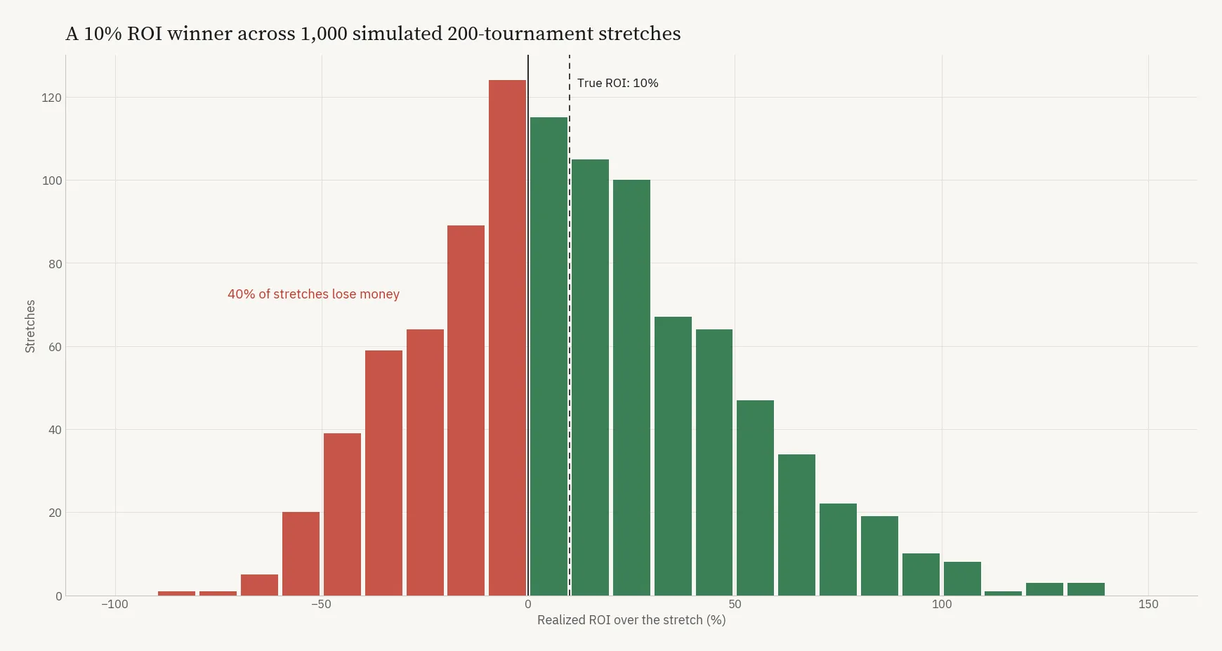
The formulas from Parts 1 and 2 still work for tournaments. The concepts hold. But plug in tournament numbers and the outputs jump an order of magnitude: bankrolls measured in hundreds of buy-ins instead of dozens, downswings measured in months instead of sessions. That scale demands different bankroll strategies, different psychological preparation, and a different relationship with your results.
The Distribution Problem
Cash game results over large samples approximate a normal distribution: a symmetric bell curve centered on your expected value. Tournament results do not. They follow a heavily right-skewed distribution, meaning that the vast majority of individual outcomes cluster on the left side (losses equal to your buy-in) while a small number of extreme positive outcomes stretch far to the right (deep runs, final tables, victories).
In a typical large-field MTT, you lose your entire buy-in roughly 80 to 85% of the time. Of the 15 to 20% of the time you cash, most cashes are small, often just 1.5 to 3 times your buy-in. The meaningful profits come from a handful of deep runs that might return 20x, 50x, or 100x+ your buy-in. This shape means that most of your lifetime tournament earnings will come from a tiny fraction of the tournaments you enter.
Consider a player with a 15% ROI who plays 1,000 tournaments at $100 each. Their expected total profit is $15,000. But that $15,000 arrives as long stretches of losing buy-ins punctuated by occasional scores that more than compensate. Remove the top 5 results from those 1,000 tournaments and the player might be breakeven or negative over the remaining 995. That concentration of returns in a few events is the defining feature of tournament variance and the reason it breaks most players' intuition about their results.
How ICM Warps the Variance Experience
There is an additional layer to tournament variance that cash games don't have: ICM (the Independent Chip Model). In cash games, every chip is worth the same amount of money. Double your stack and you've doubled your money. In tournaments, chips have diminishing marginal value. Doubling your stack does not double your equity in the prize pool. Losing half your stack costs more equity than gaining an equivalent amount adds.
This asymmetry means that the "true" variance of your tournament results, measured in dollars of equity rather than chips, is even wider than the chip-count variance suggests. A coin flip for your tournament life is a negative-equity proposition in most tournament situations, even though it's a neutral-equity proposition in chips. The ICM tax on variance is why solid tournament players avoid marginal all-ins near pay jumps and why the best players accumulate chips through smaller pots and positional play rather than gambling for stacks.
For the reader who wants to explore ICM equity calculations in specific scenarios, the Primedope ICM Calculator (https://www.primedope.com/icm-deal-calculator/) models deal scenarios and equity distributions at final tables.
ROI vs. ITM Rate
ITM (in the money) percentage is one of the most tracked and most misleading statistics in tournament poker. A player can increase their ITM rate by playing tighter on the bubble, nursing a short stack into the money rather than taking high-variance spots that build a stack for a deep run. The problem is that this strategy destroys ROI. The difference between min-cashing (1.5x buy-in) and a final table (20x to 100x+ buy-in) is so enormous that sacrificing deep run equity to secure a min-cash is one of the worst strategic trades in poker.
The only metric that matters for assessing tournament profitability is ROI: (total winnings minus total buy-ins) divided by total buy-ins. And even ROI requires an enormous sample to stabilize, a point we'll quantify in Chapter 8.
The Bink Problem
A "bink" in poker slang is a large tournament score, usually a win or deep run in a significant event. The bink problem is this: a single large score can make a losing player's results look positive for months or years afterward.
A player who enters 500 tournaments at $200 each ($100,000 in buy-ins) and ships one event for $60,000 while losing the other 499 entries has results of $60,000 minus $100,000, which is negative $40,000. But what if the score was $120,000? Now the results are positive $20,000, which looks like a 20% ROI over $100,000 in buy-ins. The player appears to be a strong winner. But their non-bink results are negative $80,000 over 499 tournaments. The entire "profit" is one event.
Every poker community has players whose lifetime graphs are essentially one spike followed by a long downward slope, with the spike large enough to keep the cumulative line above zero. They are counted as "winning players" in the statistics, and many of them believe they are, because they confuse the presence of a large score with proof of edge.
The math is simple: if you removed the player's single best result and they're deeply negative, the sample is telling you almost nothing about their true ROI. The bink might be evidence of a good player who got their due, or it might be a recreational player who got lucky once in a large field. At 500 tournaments, the data cannot distinguish between the two.
Elite Players Cash 15 to 20 Percent of the Time
This number surprises recreational players but is fundamental to understanding tournament poker. In a 1,000-runner MTT that pays 15% of the field, the best player in the world will still miss the money roughly 80% of the time. Their edge expresses itself through deeper average finishes when they do cash, and through a marginally higher cash rate that is almost invisible over small samples.
An elite player might cash 18% of the time in a field where the average is 15%. That 3-percentage-point edge is nearly undetectable over 200 or even 500 tournaments. But applied to thousands of events, it compounds into significant positive ROI through a combination of slightly more cashes and substantially deeper cashes.
The emotional reality of tournament poker is that you will lose for extended periods as a matter of mathematical certainty. Coming to terms with that is a prerequisite for playing the format at all.
You can simulate these dynamics with your own tournament parameters using the Primedope MTT variance calculator (https://www.primedope.com/tournament-variance-calculator/).
Chapter 8: Realistic ROIs in 2026
The most expensive mistake tournament players make is overestimating their ROI. The damage shows up away from the table, in bankroll decisions, lifestyle decisions, and years spent grinding a schedule that the math says cannot sustain them.
The Mechanisms Behind ROI Overestimation
There are several mechanisms and they compound.
Players remember their scores more vividly than their entries. The $15,000 Sunday major win lives in memory. The 200 buy-ins that preceded it fade into background noise. When players mentally tally their results, the highlights are overweighted and the grind is underweighted.
Players calculate ROI over favorable stretches. A player who runs their numbers from the last big score forward will see an inflated ROI. A player who runs their numbers from two years ago, including the long dry stretch before the score, will see a very different number. Both calculations are technically correct over their respective windows, but only the longer one approximates the true ROI.
Players compare themselves to publicly reported results from softer eras. The tournament scene in 2026 is dramatically tougher than it was in 2010 or 2015. Solver-assisted study, coaching programs, and mass training content have raised the baseline skill level across all stakes. A 30% ROI that was achievable at $50 buy-ins in 2012 may be 10 to 15% in 2026, and the player using the older benchmark for their bankroll and lifestyle calculations is operating on stale data.
What ROIs Look Like in Practice
What is a realistic poker ROI? The following ranges come from staking operations tracking hundreds of players across tens of thousands of tournaments. They are the tournament poker ROI numbers that survive 2,000 or more tournaments of reality.
Global-pool low stakes ($5 to $30 buy-ins, PokerStars/GGPoker):
Sustainable ROI for a strong player: 15 to 30%
Average field size: 500 to 5,000+
Competition level: moderate to tough (rising every year as training material proliferates)
Global-pool mid stakes ($50 to $200 buy-ins):
Sustainable ROI for a strong player: 8 to 20%
Average field size: 200 to 2,000
Competition level: tough (most players at this level are studying seriously)
Global-pool high stakes ($500+ buy-ins):
Sustainable ROI for a strong player: 3 to 12%
Average field size: 50 to 500
Competition level: elite
Fenced markets (Ozoon, Ignition, anonymous tables):
Sustainable ROI: generally higher than equivalent global-pool stakes
Reason: recreational players protected by anonymity, fewer regs, less data mining
Tradeoff: smaller fields, less volume availability
Crypto/alternative platforms (CoinPoker, BCPoker):
Similar dynamics to fenced markets. Softer fields, smaller sample of grinders, less HUD usage.
CoinPoker's combination of competitive rake (among the lowest at micro stakes based on our rake database of 645 data points across 18 networks) and a crypto-native player base produces particularly soft fields at low-to-mid stakes. At higher stakes, sites like ACR become more competitive on rake structure.
The planning baseline: Whatever ROI you believe you have, subtract five percentage points for bankroll and lifestyle decisions, and subtract ten if your sample is under 1,000 tournaments. If the math still works at the reduced number, you're on solid ground. If it only works at your optimistic estimate, you're one extended downswing away from a crisis.
The Tournament Sample Size Problem
The sample size problem from Chapter 2 is dramatically worse for tournaments because each "data point" (one tournament) contains far less information than 100 hands of cash games.
A cash game player might accumulate 100,000 hands in two months of serious play. A tournament grinder playing a full weekly schedule of 40 events might need two years to reach 4,000 tournaments.
At 500 tournaments with a true ROI of 20%, the standard deviation of the observed ROI is approximately 80 to 100 percentage points. This means the 95% confidence interval for the observed ROI after 500 tournaments spans from roughly negative 140% to positive 180%. Five hundred tournaments, which might represent an entire year of full-time play, cannot reliably tell you whether you're a 20% ROI winner or a losing player.
At 2,000 tournaments, the confidence interval narrows to roughly plus or minus 80 percentage points at the 95% level. This is an improvement, but the range is still enormous compared to the actual ROIs being measured (10 to 30%).
At 500 tournaments, which might represent an entire year of full-time play, the data cannot tell you whether you're a 20% ROI winner or a losing player.
The practical implication: most tournament players will never play enough events to statistically confirm their ROI with confidence. Keep tracking your results, but treat your observed ROI with deep skepticism and base your bankroll and lifestyle decisions on conservative estimates rather than peak-sample numbers.
Chapter 9: Variance Profiles by Field Size and Format
Tournament formats are not monolithic. A 50-player sit-and-go, a 500-player nightly, and a 5,000-player Sunday major produce fundamentally different variance experiences. Understanding these differences is essential for building a schedule that matches your bankroll and risk tolerance.
Small Fields (Under 100 Players)
Small-field tournaments have the lowest variance of any MTT format. The payout structures are flatter (a higher percentage of the buy-in goes to the top), the time to reach the money is shorter, and the probability of cashing is higher.
In a 45-player SNG paying the top 7, a strong player might cash 20 to 25% of the time, compared to 15 to 18% in a 1,000-runner event. The distribution of results is less extremely right-skewed because the maximum payout (a win) is typically only 10 to 15 times the buy-in rather than 100x or more.
Expected bankroll requirement: 50 to 80 buy-ins for a solid edge
Expected worst drawdown over 600 tournaments: approximately 40 to 60 buy-ins
Small-field specialists can sustain themselves with smaller bankrolls, but the trade-off is lower expected earnings per event and lower upside. The 100x score that defines the MTT experience simply doesn't exist in small fields.
Medium Fields (100 to 500 Players)
This is where most online tournament grinders spend most of their time. The nightly $55 with 300 runners, the afternoon $22 with 200 runners, the turbo $100 with 150 runners.
The variance is meaningfully higher than small fields. The payout structures become more top-heavy (first place might be 50 to 80 times the buy-in), the probability of cashing drops to 15 to 18%, and the distribution becomes more right-skewed.
Expected bankroll requirement: 80 to 120 buy-ins for a solid edge
Expected worst drawdown over 600 tournaments: approximately 80 to 120 buy-ins
A drawdown of this size can exceed the player's entire expected annual profit. A player grinding $50 buy-ins with 100 buy-ins in their bankroll ($5,000) who hits an 80 buy-in downswing ($4,000) is facing a near-ruin event despite playing well. That is a mathematically expected outcome over a sample of a few hundred tournaments.
Large Fields (500+ Players)
Sunday majors, guaranteed prize pool events, and series tournaments. Field sizes of 1,000 to 10,000+.
This is where tournament variance reaches its most extreme expression. First place payouts can exceed 200 times the buy-in in fields over 5,000. The probability of any individual cash is 12 to 15%. The distribution of results is so right-skewed that a player can play 1,000 of these events and have their cumulative profit determined almost entirely by one or two results.
Expected bankroll requirement: 100 to 200+ buy-ins for a solid edge
Expected worst drawdown over 600 tournaments: approximately 100 to 150 buy-ins
The numbers at this level can seem absurd. A 200 buy-in bankroll at $100 average buy-in is $20,000, and even that provides no guarantee of surviving. But the upside is proportionally enormous: a single deep run can return the equivalent of hundreds of buy-ins.
Large-field tournaments are not for the underfunded. Players who enter Sunday majors without appropriate bankrolls are playing a game where the math almost guarantees they will go broke before their edge (if it exists) has time to manifest.
SNGs and Spins
Sit-and-go formats (traditional SNGs and spin-and-go/blast formats) have their own variance characteristics.
Traditional SNGs (6 to 45 players): Lowest variance in tournament poker. Standardized structures, small fields, predictable payout distributions. A strong player can sustain on 40 to 80 buy-ins.
Spins/Blasts (3-player hyper-turbo with randomized prize pools): Extremely high variance due to the lottery-style prize distribution. A significant portion of the expected ROI comes from hitting the occasional large multiplier, and the frequency of those multipliers means very long stretches of negative results are normal. Bankroll requirements: 200+ buy-ins for even a strong edge, and the concept of "proving" you have an edge requires tens of thousands of events.
Blind Structure Speed
Not all tournaments with the same field size produce the same variance. Turbo and hyper-turbo structures compress the decision tree: shorter levels mean fewer postflop decisions, more preflop shove-or-fold situations, and less room for skill to express itself in individual hands. The result is higher variance for a given field size and ROI.
Deep stack tournaments with longer levels do the opposite. More postflop play means more decisions per tournament, which gives skilled players more opportunities to realize their edge and produces a slightly narrower distribution of outcomes.
The practical implication for bankroll management: if your schedule is heavy on turbos, budget for the higher end of the bankroll ranges in the tables above. If you primarily play deep stacks, the lower end may be adequate. A mixed schedule falls somewhere in between.
Mixed Schedules and Portfolio Diversification
Most serious tournament players don't specialize in a single field size. They play a mix of small, medium, and large-field events, often combined with SNGs or satellites. This mixing has a natural diversifying effect on variance, similar to diversifying a financial portfolio.
A player who splits their schedule between 200-runner events and 2,000-runner events will have lower total variance than a player who only plays the 2,000-runner events, assuming the same total buy-in expenditure. The smaller events provide a more consistent return (smaller but more frequent cashes) that cushions the long losing stretches inherent in the large-field events.
The portfolio approach to tournament scheduling: build your core volume from medium-field events where your edge is most consistent and your results converge fastest. Add large-field events for upside, but recognize them as the high-variance portion of your "portfolio" and don't let them take over your schedule unless your bankroll can absorb the swings.
Chapter 10: The True Cost of a Tournament Downswing
Cash game downswings are measured in big blinds lost and hours played below expectation. Tournament downswings are measured in months of life spent losing money while paying living expenses. This chapter quantifies that cost because understanding it prevents the two most common career-ending mistakes: quitting during a survivable downswing and continuing during a non-survivable one.
What a Normal Tournament Downswing Looks Like
How long does a poker downswing last? For a tournament player with a genuine edge, a five-month stretch of negative results is a routine event, one the math predicts will happen to almost every full-time grinder at least once per year. Here is what it looks like in concrete numbers.
Timeline: Over 12 months, the player enters approximately 2,500 tournaments ($125,000 in buy-ins). Their true ROI is 15%, so their expected profit is $18,750.
During months 3 through 7 (a five-month stretch within the year), the player hits a sustained cold run. No final tables, a below-average number of cashes, and the cashes that do come are min-cashes rather than deep runs. The player's cumulative results during this stretch show a loss of approximately $15,000 to $20,000 in buy-ins against a breakeven return.
During this five-month stretch, the player is also paying $3,000 per month in living expenses. The total cash drain over those five months is the buy-in losses plus $15,000 in living costs: roughly $30,000 to $35,000 out of pocket. If the player started the year with a $20,000 bankroll, they may be facing ruin while playing winning poker, simply because the variance timeline outlasted their financial runway.
The Cash Flow Problem
The math of tournament variance creates a cash flow problem that doesn't exist in cash games. A cash game player with a positive win rate generates a roughly positive expected cash flow every month, even if individual months are negative. The expected value is always positive, and the variance is moderate enough that long stretches of negative cash flow are rare for a properly rolled player.
A tournament player with a positive ROI can easily generate negative cash flow for three, six, or even twelve months in a row. The expected value per month is still positive, but the variance is so enormous relative to the edge that the monthly expected value can be dwarfed by the monthly standard deviation. A player whose monthly expected profit is $2,000 but whose monthly standard deviation is $8,000 will have many, many months where the actual result is negative, even over a career where the cumulative result is strongly positive.
How to Calculate Your Personal Runway
The critical planning exercise for any aspiring tournament professional:
Step 1: Estimate your monthly living expenses (rent, food, health insurance, transportation, subscriptions, taxes on estimated winnings). Be honest. Underestimating this number is the single most common reason tournament careers end prematurely.
Step 2: Estimate your monthly expected tournament profit based on your realistic ROI (use the conservative planning baseline from Chapter 8: your observed ROI minus 5 to 10 percentage points) and your monthly buy-in investment.
Step 3: Estimate the duration of a plausible downswing from the profiles in Chapter 9. For medium-to-large field grinding, assume you will face a 100+ buy-in downswing at some point during any 12-month period.
Step 4: Calculate your total cash requirement: your tournament bankroll (100 to 200 buy-ins) PLUS your living expenses for the duration of an expected downswing PLUS a safety margin for the downswing being worse than expected (add 20 to 30%).
If the total exceeds your available resources, the arithmetic says you cannot responsibly go full-time at those stakes yet. Grinding part-time at lower stakes while holding a job that covers living expenses, playing higher stakes on weekends only, or building your bankroll at lower stakes before taking the full-time shot are all sound paths. The costly path is skipping the math and discovering the answer two years and $50,000 too late.
When to Quit, When to Drop Down, and When to Push Through
This is the decision most tournament players get wrong, because the decision requires distinguishing between a normal downswing (push through), a bankroll emergency (drop down), and a permanent edge loss (consider quitting the format or stakes).
Push through when: your bankroll is above the minimum required for your stakes at your target risk of ruin, your play quality is not degraded (Chapter 11), and the downswing duration is within the range you planned for.
Drop down when: your bankroll falls below the minimum for your current stakes, even if you believe the downswing is temporary. Moving down preserves the bankroll so it can grow back. Continuing to play stakes you're no longer rolled for is how temporary downswings become permanent ruin.
Consider a fundamental reassessment when: the downswing exceeds the duration and depth of what the math predicts for your assumed ROI by a significant margin (more than two standard deviations), or when an honest review of your play reveals that your edge has eroded due to changes in the player pool, personal factors, or failure to keep up with evolving strategy.
Chapter 11: Maintaining Your Edge During a Downswing
Variance is external and uncontrollable. Your edge is internal and, in theory, stable. But in practice, downswings erode the very edge that allows you to survive them, creating a feedback loop that can turn a recoverable variance event into a career-ending spiral.
The Doom Loop
The sequence is predictable and plays out at every level of tournament poker, though the speed and severity vary by player:
Phase 1: The downswing begins and results fall below expectation. The player recognizes this as variance and maintains their normal game.
Phase 2: The downswing continues longer than the player expected. Frustration begins to accumulate. The player starts pressing: taking slightly more marginal spots to "get unstuck," entering higher buy-in events to recover faster, playing longer sessions despite fatigue.
Phase 3: The pressing behavior introduces actual leaks. Aggression that was once edge-based becomes emotion-based. Marginal bluffs increase. Fold frequency in spots where patience is correct decreases. The player's actual ROI drops, meaning the downswing is now partly variance and partly degraded play.
Phase 4: The player recognizes (or suspects) that their play has degraded, which adds anxiety to the frustration. Self-doubt compounds. Some players respond by studying more, which can help. Others respond by playing more volume, which accelerates the leak introduction.
Phase 5: The player either breaks the cycle (takes a break, addresses the leaks, returns to baseline play) or the cycle breaks the player (bankroll depleted, mental health degraded, career reconsidered).
The doom loop is dangerous because it converts a survivable variance event into an unsustainable one. A player with a 15% ROI and a 150 buy-in bankroll can survive a 100 buy-in downswing mathematically. But if the doom loop reduces their effective ROI to 0% during the downswing (through degraded play), the math changes entirely.
Signs Your Play Is Degrading
The following indicators are observable in your tracking data and in honest self-assessment. If three or more are present simultaneously, the doom loop is active:
Your average buy-in has crept up as you enter higher stakes to chase losses. Session length has increased without a corresponding increase in volume targets. VPIP or PFR has shifted meaningfully from your established baseline. Play happens in time slots you normally avoid (late night, early morning, tilted sessions). Study time that was previously consistent gets skipped, and hands from recent sessions go unreviewed. Tournament registrations happen without checking whether they fit your bankroll requirements. Before sitting down to play, your mood is consistently negative or anxious rather than focused.
How to Break the Cycle
The interventions are simple to describe. Implementing them during a downswing, when your emotional state is compromised, is the hard part.
Reduce volume temporarily. Cutting your weekly tournament count by 30 to 50% during a downswing preserves bankroll and creates space for the emotional reset that prevents the doom loop from progressing. The counterargument ("but I need the volume to recover") is mathematically true but psychologically wrong. Volume at degraded play quality accelerates ruin.
Reduce stakes if your bankroll requires it. If your bankroll no longer supports your current buy-in level at your target risk of ruin, moving down is the mathematical requirement. The emotional resistance to moving down is one of the most dangerous impulses in a poker player's psychology.
Return to study with a focus on specific leaks. Pull up your tracker and identify the three biggest leaks by expected value. Fix those. General theory study during a downswing can become an avoidance mechanism (studying feels productive without requiring you to confront the specific ways your play has degraded).
Set a poker stop loss based on decision quality. Instead of "I'll quit if I lose 5 buy-ins," use "I'll quit if I notice myself making decisions I wouldn't make during the first hour of play." The former is results-based and can encourage passive play to avoid the stop loss. The latter targets the actual problem.
Talk to other serious players. The isolation of online poker amplifies the doom loop. Other grinders who have survived downswings can provide perspective that no amount of self-talk can replicate. If you have access to a coaching community or staking group, this is when it earns its value.
Chapter 12: Tournament Bankroll Requirements, the Complete Guide
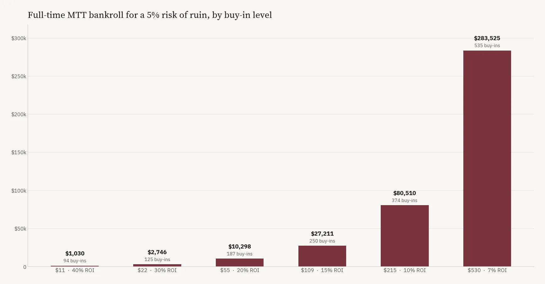
What follows is the practical reference for tournament bankroll requirements: specific numbers by stake level, the difference between life bankroll and playing bankroll, and the unique math of satellite strategy.
The Bankroll Table
The following table assumes standard online payout structures where approximately 15% of the field is paid with typical top-heavy weighting. Flatter payout structures (more money spread across more places) reduce variance and the bankroll requirement. More top-heavy structures increase both.
| Average Buy-In | Assumed ROI | Minimum Bankroll (5% RoR) | Conservative Bankroll (2% RoR) | Recommended |
|---|---|---|---|---|
| $5-$15 | 20-30% | 60-80 buy-ins | 100-120 buy-ins | 80 buy-ins |
| $20-$50 | 15-25% | 80-100 buy-ins | 120-150 buy-ins | 100 buy-ins |
| $50-$100 | 10-20% | 100-120 buy-ins | 150-200 buy-ins | 150 buy-ins |
| $100-$300 | 8-15% | 120-150 buy-ins | 200-250 buy-ins | 200 buy-ins |
| $500+ | 5-12% | 150-200 buy-ins | 250-300 buy-ins | 250 buy-ins |
The "Recommended" column accounts for the reality that your actual ROI is uncertain, your living expenses create cash flow pressure during downswings, and the consequences of going broke at each level are increasingly severe.
Life Bankroll vs. Playing Bankroll
How much money do you need to play poker full time? The playing bankrolls in the table above are only part of the answer. For a part-time player with a separate income source, the playing bankroll is the only number that matters. For a full-time tournament professional, the total capital requirement is a different calculation entirely, and it is almost always larger than the player expects.
A full-time pro needs:
Playing bankroll: per the table above.
Living expense runway: 6 to 12 months of living expenses held separately from the playing bankroll. This money is for rent, food, insurance, and bills during downswings when tournament income is zero or negative.
Emergency fund: 3 months of expenses beyond the runway, for genuine emergencies (medical, car, etc.) that occur during a downswing.
Example: A full-time grinder playing $100 average buy-in with $3,000 monthly living expenses.
Playing bankroll: $15,000 (150 buy-ins)
Living expense runway: $36,000 (12 months)
Emergency fund: $9,000
Total cash requirement: $60,000
To responsibly grind $100 average buy-in MTTs full-time, a player needs $60,000 in total capital. Most players who attempt it underestimate the requirement by a factor of two or three.
Poker as a full-time income source requires capital that most players, even genuinely winning ones, don't have before they attempt it. The shortfall stays invisible until the first extended downswing, and then it shows up as ruin.
Satellite Bankroll Strategy
Satellites (tournaments where the prize is an entry into a larger event rather than cash) have a unique variance profile that can be exploited for bankroll efficiency.
In a standard satellite paying the top 10% of the field with identical prizes (a seat in the target event), the payout structure is dramatically flatter than a normal MTT. There's no difference between finishing 1st and finishing 10th: you all get the same seat. This flatness reduces variance substantially.
A strong player's edge in satellites often exceeds their edge in the corresponding direct buy-in events, because satellite strategy is more forgiving of small mistakes (survival-oriented play near the bubble is simpler than ICM-optimized play in a normal tournament) and because the flat payout structure means the edge compounds more predictably.
The bankroll implication: if you can maintain a 30% or higher ROI in satellites to a $500 event, it may be more bankroll-efficient to satellite into those events than to buy in directly, even if your direct buy-in ROI is positive. The lower variance of the satellite path means your bankroll faces less drawdown risk per entry into the larger event.
The strategic trap: some players become satellite specialists who never play the target events. They win seats and sell them or unregister for the cash equivalent. If your goal is bankroll building, this can be rational. If your goal is developing as a tournament player, you need the experience of playing the larger events, and a shelf of unplayed seats gets you none of it.
Part 4: Practical Applications
Chapter 13: Diagnosing Your Results
The formulas and frameworks from Parts 1 through 3 are predictive: given your parameters, what should you expect? This section inverts the question. Given your results, what can you conclude, and what should you do next?
The All-In EV Adjusted Line
Every major tracking tool displays an "all-in EV adjusted" line alongside your actual results. In PokerTracker 4, it's the green line on your results graph. In Hand2Note, toggle the EV line in the graph panel options.
This line recalculates your results by replacing each all-in showdown result with the expected value of the hand at the moment all the money went in. If you got all-in with 80% equity and lost, the EV line credits you with 80% of the pot instead of zero. Over time, the EV line strips out the luck component of all-in situations and shows what you "should have" won.
The EV line is useful but incomplete. It captures luck in all-in pots but misses several important variance sources:
Preflop and postflop runouts where no one was all-in (you had the best hand on the flop but a scare card came on the turn and your opponent folded to your bet, or vice versa). These outcomes affect your actual results but are not captured in the all-in EV calculation.
Cooler frequency (how often you get dealt a strong hand against a stronger hand). Being dealt KK against AA is not reflected in the EV line until the money goes in.
Opponents' mistakes that happened to work out. If an opponent called your river bet with a bad hand and happened to hit a two-outer on the river, that bad call reduced your EV line by the amount you "should have" won, but the opponent's underlying mistake is still a long-term profit source for you.
Treat the all-in EV line as a directional indicator. If your actual line is significantly below your EV line over a large sample, you are running below expectation in all-in pots. If it's above, you're running above. But the gap doesn't tell you whether the non-all-in components of your results are also running above or below expectation.
A Diagnostic Checklist
When you suspect your results don't reflect your true ability, work through these steps:
Step 1: Check the EV line. Is the difference between actual results and EV-adjusted results large relative to your expected earnings? If so, a significant portion of your downswing (or upswing) is attributable to all-in luck.
Step 2: Compare your stats to your historical baseline. Look at VPIP, PFR, 3-bet %, fold-to-3-bet, WTSD (went to showdown), W$SD (won money at showdown), and aggression frequency. If these numbers have drifted from your established baseline, your play has changed, and that change may be contributing to or masking variance effects.
Step 3: Review your largest pots. Sort by pot size and look at the 20 biggest pots over the period in question. Are you consistently getting the money in good (the EV line confirms this)? Or are you making large mistakes that inflate the pot before showdown?
Step 4: Calculate the expected range of outcomes. Given your win rate, standard deviation, and the number of hands in your sample, what range of cumulative results is consistent with your parameters? If your actual results fall within the 95% confidence interval of your expected results, the downswing (or upswing) is within normal variance. If the stretch exceeds what the math predicts at reasonable confidence levels, either your true win rate has changed (the games got tougher, you moved stakes, your edge eroded) or you're playing below your actual ability. You can run this calculation with your exact parameters using the Primedope poker variance calculator (https://www.primedope.com/poker-variance-calculator/). Enter your win rate, standard deviation, and number of hands, and the calculator shows you the full range of outcomes consistent with your data.
Step 5: Assess environmental changes. Has the player pool changed? Have you moved to a different time slot? Has a key recreational player left the regular game? Have rake or reward structures changed? Environmental changes can reduce your true win rate without any change in your play quality.
Tournament-Specific Diagnostics
Tournament results are harder to diagnose because the sample sizes are smaller and the variance is larger. But there are still useful indicators:
ICM pressure spots. Review your play in critical spots near the bubble and at final tables. Are you consistently making ICM-correct decisions, or are you calling too loose (destroying equity) or folding too tight (sacrificing chip accumulation equity)?
Final table play. If you're making many final tables but finishing poorly (7th to 9th in a 9-handed final table), your short-handed play may need improvement. If you're rarely making final tables despite a healthy ITM rate, your pre-final-table play may be too passive (surviving to the money but arriving with a short stack).
Bubble decisions. Are you exploiting the bubble when you have a big stack? Are you folding too much when short? These spots have outsized impact on long-term results because the equity swings are large relative to any single pot.
Satellite performance. If satellites represent a significant portion of your schedule, track their results separately. Your overall ROI is a blend of satellite and direct buy-in results, and the blend can mask significant differences in performance across the two formats.
Chapter 14: The Psychology of Variance
Knowing the math doesn't make the experience easy. Understanding that a 100 buy-in downswing is within normal parameters doesn't prevent it from feeling catastrophic when you're living through it. What follows is an account of the cognitive patterns that make variance harder than it needs to be, and the practical responses that protect your decision-making.
The Biases That Make Variance Worse
Loss aversion. You already know this one in your gut: losing $500 hurts more than winning $500 feels good. Roughly twice as much, according to the research. In poker, this means your downswings occupy more mental real estate than your upswings, even when the upswings were larger. A month where you lost $3,000 will feel more significant than a month where you won $4,000, even though the net over two months is positive $1,000. Your brain keeps a running emotional tally that is structurally biased toward the negative.
The countermeasure is numerical tracking: look at the graph over 6 or 12 months instead of the last session, set a review schedule (weekly or monthly), and base decisions on that review rather than on the post-session emotional state.
Recency bias. Your last ten sessions feel more real than your last two hundred. This means a player in the middle of a downswing will overweight the downswing's severity relative to their longer track record, and a player on a heater will overweight the heater. Both states distort decision-making: the downswing player makes conservative, fear-based decisions ("I should move down, I should tighten up, I should stop taking shots"), while the heater player makes aggressive, confidence-based decisions ("I should move up, I'm ready for higher stakes, I should increase my schedule").
The countermeasure: anchor all strategy and bankroll decisions to your full historical sample rather than your recent results. If your decision would be different based on your last 100 tournaments versus your last 1,000, you're being swayed by recency.
Confirmation bias. During a downswing, you notice every bad beat, every cooler, every suckout. During an upswing, you barely register them. This selective attention creates a narrative ("the site is rigged," "the cards always come against me," "I can't win a flip") that feels overwhelmingly supported by evidence because you're only cataloging evidence that confirms it.
The countermeasure: when you catch yourself building a narrative about your results, check it against the EV line and the confidence interval math. The narrative will almost always collapse when confronted with the actual numbers.
Hot hand fallacy. Poker players who believe they are "running hot" will sometimes take marginal spots they'd normally avoid, reasoning that the momentum will carry them. Poker players who believe they are "running cold" will sometimes fold strong hands in marginal spots, reasoning that they'll lose anyway. Neither belief has mathematical basis. Cards have no memory, and the probability of winning the next flip is 50% regardless of the last twenty.
The countermeasure: make every decision on the current hand's expected value, with the results of previous hands carrying no weight. This is easy to state and extraordinarily difficult to practice consistently, which is why the best players treat it as a discipline rather than an attitude.
When to Stop Playing
A stop-loss based on results (quitting after losing three buy-ins) can cost EV if you're playing well in a good game. The better trigger is decision quality: how do you know when it has degraded to the point where continuing to play is negative EV?
The honest indicators: you are reacting emotionally to outcomes instead of evaluating each decision on its merits. Calls or folds go in that you know are incorrect at the time you make them. Play speeds up, with decisions clicked through without full consideration. Additional tables get opened, or additional tournaments entered, without conscious evaluation. Anger surfaces at specific opponents, at the site, or at yourself.
If you recognize two or more of these, stop. Not because you've lost a certain amount, but because your edge has temporarily evaporated. A session played at reduced quality depletes bankroll, deepens the downswing, and reinforces the emotional patterns that caused the degradation in the first place.
Planning the Session Before It Starts
The "when to stop" framework above is reactive. A proactive complement: decide before you sit down how long you intend to play and under what conditions you'll extend or cut short.
Set a time frame that matches your typical window of peak performance: a player who knows from experience that their decision quality degrades after four hours plans a four-hour session. If you're running well in a soft game at hour three, extend. When you're grinding through tough tables at hour two and already checking your phone between decisions, cut it short. The pre-commitment makes the mid-session decision easier because you're comparing reality against a plan instead of improvising the call in the moment.
Tilt as a Variance Amplifier
Tilt deserves special treatment because it creates a feedback loop with variance. Variance causes tilt. Tilt increases variance (through larger pots played with reduced edge) and decreases win rate simultaneously. The combined effect is that a tilted player's results diverge from their normal results far faster than pure variance would produce.
Quantifying the effect: if tilt reduces your win rate from 4 bb/100 to 1 bb/100 (a modest degradation; some players lose far more) and your standard deviation stays at 90 bb/100, your risk of ruin at 40 buy-ins jumps from 1.9% to 13.9%. That's the damage from a 3 bb/100 win rate reduction. The psychological components, increased aggression, larger average pot sizes, decreased fold discipline, can push the effective standard deviation higher as well, compounding the damage.
Poker tilt management is a bankroll management tool with quantifiable financial impact. Every session played on tilt has a measurable cost in expected value, and over a career, those costs can exceed the impact of rake. The doom loop described in Chapter 11 is tilt at its most systematic: a sustained degradation that converts a survivable downswing into a threatening one.
The most effective tilt reduction strategy is awareness plus predetermined rules. Know your tilt triggers (bad beats, specific opponents, session duration, life stress). Set rules for each trigger before you start playing ("if I take a bad beat in a pot over X buy-ins, I will take a 5-minute break before playing the next hand"). Follow the rules mechanically, especially when they feel unnecessary, because the urge to break them is strongest in the moments they were written for.
Chapter 15: Reducing Variance Without Reducing Edge
You can reduce variance without giving up your edge, within limits. The methods are more mundane than most players expect. They are a series of decisions, most of them made away from the table, that shift your variance profile without sacrificing expected earnings, and in some cases while increasing it.
Game Selection
No single decision reduces variance more than game selection, and most players spend almost no time on it.
Against a table of regulars, your profit comes from thin 3-bet pots and marginal river decisions where you're right 55% of the time. One session you're up three buy-ins from a well-timed bluff catch; the next you're down four because the river bricked twice in spots where you were slightly ahead. Against a table with two recreational players, your profit comes from value betting three streets against someone who calls with third pair. The win rate might be similar, but the day-to-day experience is completely different.
The variance reduction comes from the composition of your winning pots. Against weaker players, a higher proportion of your profit comes from clear-cut situations with strong equity advantages, spots where you're a 70% or 80% favorite rather than a 55% favorite. These spots produce a more consistent stream of wins compared to the thin-margin, high-variance spots that characterize tough lineups.
The practical framework: track your win rate by table type (number of recreational players, average VPIP of the table) if your tracking software supports it. Most players will find that their hourly EV is dramatically higher at tables with at least one recreational player, and their standard deviation is meaningfully lower.
Table Selection
Within any given site, table selection is the micro version of game selection. Cash game players who use lobby stats, waiting lists, or seat scripts to find the softest available tables are making a variance management decision on top of a win rate decision. Sitting at a table with one recreational player instead of zero changes your session's expected distribution of outcomes. This is most impactful in games where table selection tools are available, which includes most sites except those with anonymous seating. On anonymous sites, the trade-off is different: you can't select your table, but the overall pool tends to be softer because the recreational players are protected from being targeted.
Site Selection
Where you play is as much a variance decision as what you play. Sites with softer player pools, better rake structures, or higher rakeback provide both a higher effective win rate and a more favorable variance profile, as demonstrated in Chapter 5.
Sites with anonymous tables (Ozoon, Ignition) offer a particular variance advantage: the inability to identify and exploit specific opponents means that the games play softer on average, because recreational players are not hunted and driven away as quickly. The trade-off is that you also cannot exploit specific tendencies of identified opponents, which may reduce your maximum win rate compared to a tracked environment.
Crypto-native platforms (CoinPoker, BCPoker) tend to attract a different player demographic: more recreational crypto enthusiasts, fewer grinders with tracking software. At low-to-mid stakes, this can produce both a higher win rate and lower effective variance.
Poker site selection for winning players is a variance management decision. Choose by analysis using the Primedope poker rake calculator (https://www.primedope.com/online-poker-rake-comparison-rake-calculator/), recheck periodically, and be willing to move when the math justifies it.
Format Selection
If you play multiple formats, you can adjust your format mix to manage your overall variance exposure.
Full ring NLHE has the lowest standard deviation of any common online format (60 to 80 bb/100). Six-max is moderately higher (75 to 120). PLO is dramatically higher (120 to 160). Shifting volume from PLO to NLHE 6-max reduces variance; shifting from NLHE to full ring reduces it further. Of course, these shifts also affect your win rate and hourly EV, so the trade-off is not free.
For tournament players, the same principle applies to field size. Shifting volume from large-field events (high variance, high upside) to medium-field events (moderate variance, moderate upside) reduces the severity of downswings at the cost of lower individual scores. The portfolio approach described in Chapter 9 is a variance management strategy.
Running It Twice
Available on many online platforms and in some live games, running it twice divides the pot into two halves, each decided by a separate board runout. The expected value is identical to running it once (each board is an independent event with the same equity), but the standard deviation per hand is reduced because the two outcomes partially cancel each other.
A simple example: you're all-in with 60% equity in a $200 pot. Running it once, your expected value is $120, but you either win $200 or $0. Your standard deviation on this hand is $98. Running it twice, you might win one board and lose the other ($100), win both ($200), or lose both ($0). The expected value is still $120, but the standard deviation drops to approximately $69.
The effect is modest on any single hand but compounds over thousands of hands into measurably smoother results. One caveat: running it twice can marginally change how opponents play against you. Some players call wider when they know the variance of the individual pot is reduced. Whether this costs you more EV than the variance reduction saves you in tilt prevention is player-dependent, but it's worth being aware of the dynamic.
Rake Optimization
As covered in Chapter 5, reducing your effective rake is equivalent to increasing your win rate for variance purposes. The key actions:
Compare rakeback and reward programs across sites you're considering. The Primedope Rake Calculator (https://www.primedope.com/online-poker-rake-comparison-rake-calculator/) provides this comparison using 645 data points across 18 networks.
Maximize available rakeback on your current site. Some sites offer tiered rewards where higher volume earns better rates.
Consider whether a site's rake structure favors your play style. "Net rake" systems favor tight players who contribute less to pots they don't win. Traditional rake-from-pot systems affect all players equally per pot.
Shot-Taking as Variance Management
The shot-taking framework from Chapter 6 is a variance management tool in disguise. By capping the downside of a higher-stakes attempt at a predetermined number of buy-ins, you limit your variance exposure while maintaining access to higher-stakes upside.
For tournament players, the satellite path to larger events is an analogous tool. Satelliting into a $500 event costs less in variance than buying in directly because the satellite investment is spread across multiple lower-buy-in events with flatter payout structures.
What You Cannot Do
You cannot reduce variance to zero while maintaining a positive expected value. The variance is intrinsic to the game. Every strategy that reduces variance (playing tighter, avoiding large pots, playing smaller fields) also tends to reduce the maximum expected value.
The goal is to find the point where the variance you accept is proportional to the edge you maintain and the bankroll you hold. That point is different for every player. A player with a large bankroll and high risk tolerance can afford more variance (and capture more upside). A player with a smaller bankroll or lower risk tolerance should actively manage variance toward the lower end, even at the cost of some expected value.
The math in this guide locates that point for your numbers. Holding your play there through a downswing is the hard part.
Appendices
Appendix A: Variance Formulas Quick Reference
Expected Value (Cash Games)
EV = (WR / 100) * number_of_hands * bb_value
Standard Deviation Over a Sample
SD_total = SD_per_100 * sqrt(number_of_hands / 100)
Confidence Interval (95%)
Lower = EV - (1.96 * SD_total)

Upper = EV + (1.96 * SD_total)
Risk of Ruin
RoR = e^(-2 * WR * BR / SD^2)
Where WR = win rate in bb/100, BR = bankroll in big blinds, SD = standard deviation in bb/100.
Minimum Bankroll for Target Risk of Ruin
BR = -SD^2 * ln(RoR_target) / (2 * WR)
Standard Error of Win Rate
SE = SD / sqrt(number_of_hands / 100)
Kelly Criterion (Simplified)
Optimal stakes = (WR * BR) / SD^2
Appendix B: Bankroll Requirement Quick Reference Tables
Cash Games (assuming 90 bb/100 standard deviation)
Minimum bankroll in buy-ins for 5% risk of ruin:
| Win Rate (bb/100) | Bankroll (buy-ins) |
|---|---|
| 1 | 121 |
| 2 | 61 |
| 3 | 40 |
| 4 | 30 |
| 5 | 24 |
| 6 | 20 |
| 8 | 15 |
| 10 | 12 |
For 1% risk of ruin, multiply by approximately 1.5.
For PLO (140 bb/100 SD), multiply by approximately 2.4.
Tournaments
| Average Buy-In | Assumed ROI | Recommended Bankroll |
|---|---|---|
| $5-$15 | 20-30% | 80 buy-ins |
| $20-$50 | 15-25% | 100 buy-ins |
| $50-$100 | 10-20% | 150 buy-ins |
| $100-$300 | 8-15% | 200 buy-ins |
| $500+ | 5-12% | 250 buy-ins |
Appendix C: Standard Deviation Benchmarks by Game Type
| Game Type | Typical SD Range (bb/100) | Notes |
|---|---|---|
| NLHE Full Ring (9-max) | 60-80 | Lowest common SD; tight ranges, smaller pots |
| NLHE 6-max | 75-120 | Most common online format; moderate variance |
| NLHE Heads-Up | 100-140 | Highest NLHE variance; every hand contested |
| PLO 6-max | 120-160 | Closer equities, larger average pots |
| PLO Full Ring | 100-140 | Slightly lower than PLO 6-max |
| Mixed Games (8-Game) | 90-120 | Varies by component game; PLO rounds spike SD |
| Live NLHE (1/2 to 5/10) | 120-160 | Deeper stacks, more multiway pots, irregular sizing |
| Live PLO | 150-200+ | Extreme variance; bankroll requirements are enormous |
Appendix D: Glossary
All-in EV (Expected Value): The expected value of a hand at the moment all chips are committed. Used by tracking software to create the "EV-adjusted" results line that strips out luck in all-in situations.
Bankroll: The total amount of money reserved exclusively for playing poker. Separate from living expenses and emergency funds.
Confidence interval: A range of values within which the true parameter (e.g., your true win rate) is expected to fall with a given probability. A 95% confidence interval means there is a 95% probability the true value lies within the stated range.
Downswing: A sustained period where actual results fall below expected value. Measured in buy-ins lost (tournaments) or big blinds lost (cash games) below the expected value line.
Expected value (EV): The long-run average outcome of a decision or series of decisions. In poker, your expected earnings per hand, session, or year based on your win rate.
ICM (Independent Chip Model): A mathematical model that converts tournament chip counts into prize pool equity. Critical for decision-making near pay jumps and at final tables.
ITM (In the Money): The percentage of tournaments in which a player finishes in a paying position. Often misleading as a measure of tournament skill because it can be inflated by conservative play that sacrifices deep-run equity.
Kelly Criterion: A formula for optimal bankroll allocation that maximizes long-term growth rate. In poker, it suggests the maximum stakes a player should play given their bankroll, win rate, and standard deviation.
Normal distribution: A symmetric bell-shaped probability distribution. Cash game results over large samples approximate this distribution due to the central limit theorem.
Risk of ruin (RoR): The probability of losing an entire bankroll before it grows indefinitely, assuming fixed stakes, win rate, and standard deviation. Expressed as a percentage.
ROI (Return on Investment): For tournaments, the total profit divided by total buy-ins, expressed as a percentage. A 15% ROI means the player earns $15 for every $100 invested in buy-ins, on average.
Standard deviation (SD): A measure of how far individual outcomes spread from the average. In cash games, measured in big blinds per 100 hands (bb/100). Higher SD means wider swings.
Standard error (SE): The standard deviation of a sample statistic (such as your observed win rate). Used to calculate confidence intervals around your estimated true win rate.
Variance: The square of the standard deviation. Measures the spread of outcomes around the expected value. Often used colloquially in poker to mean "the random component of results."
Win rate: The rate of profit per unit of play. In cash games, measured in big blinds per 100 hands (bb/100). In tournaments, measured as ROI (percentage return on buy-ins).
Tool Links
Primedope Poker Variance Calculator
https://www.primedope.com/poker-variance-calculator/
The poker variance calculator and simulator used by players worldwide. Enter your win rate, standard deviation, and number of hands to see 20 possible outcome paths, confidence intervals, and risk of ruin. Works for cash games at any stake or format, including PLO variance scenarios.
Primedope Tournament Variance Calculator
https://www.primedope.com/tournament-variance-calculator/
MTT variance calculator for tournament players. Enter your ROI, buy-in, field size, and number of tournaments to see the full distribution of possible outcomes over any sample.
Primedope Poker Rake Calculator
https://www.primedope.com/online-poker-rake-comparison-rake-calculator/
Online poker rake comparison across 18 networks using 645 data points. Enter your stakes and game type to see which sites offer the lowest effective rake, including rakeback and rewards.
Primedope ICM Calculator
https://www.primedope.com/icm-deal-calculator/
Model ICM equity and deal scenarios at final tables. Enter stack sizes and payout structures to calculate each player's equity in the remaining prize pool.
This guide is a living document. The formulas are permanent; the win rates, rake structures, and ROIs plugged into them are checked against current data with each edition.
About the Author
Zach Schneider has been in professional poker for 15 years, first as a player and then on the operational side of the industry. He currently manages operations and content at BBZ Poker, one of the top tournament training platforms in the world, and holds equity in BBZ Staking as an advisor, where he helps oversee a roster of 150+ tournament professionals. He owns Primedope.com, home to the variance and rake calculators this guide is built around.
That dual perspective, years of living through variance as a player followed by quantifying it daily across hundreds of careers from the staking side, is the foundation of this guide. Across a roster of 150+ players, downswings arrive on schedule, at the frequency and depth the formulas predict, and planning around them is a routine part of the job.
Primedope.com has hosted the poker world's most widely used variance calculators since 2013, cited by Wikipedia, referenced by PokerNews, and credited by GTO Wizard. This guide is the companion to those tools: the formulas behind them, worked dollar examples for every calculation, and the practical decisions the math should drive.
It covers cash games, tournaments, bankroll management, and the psychology of downswings. Each chapter is self-contained. You can read straight through or skip to the format relevant to you.
The numbers here will not flatter you. The required bankroll is larger, the sample size smaller, and the win rate less certain than most players assume.